This post describes a circuit that can detect a mains frequency AC current and translate it into a voltage that is proportional to the current. It does this while being electrically isolated from the AC current.
One way of measuring the current to a single phase AC load, like a motor or a heater, is to use a current sense transformer around a wire that conducts the current. One kind of current sense transformer is the Rogowski coil, which is basically an air-core toroidal coil where one of the leads is routed back inside the coil to end up on the same side as the other lead. The absence of an iron/ferrite core makes the Rogowski coil immune to saturation, so it can handle large currents while still being linear.
The output voltage of the coil is proportional to the rate of change of the current to be measured, so in order to get a voltage proportional to the current itself, one has to use an integrator. If the current is known to be a sinusoid of a fixed frequency, it is not necessary to integrate the voltage as a simple factor determines the relationship between the current and the coil voltage, but such a design would make the circuit very sensitive to high-frequency overtones. The circuit discussed here contains an integrator so that it gives accurate outputs for a wide range of frequencies.
Below is a schematic of the integrator circuit I came up with.
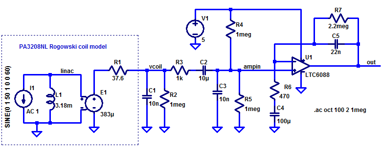
The components in the box to the left is a simulation model of the Rogowski coil PA3208NL. This device has an internal resistance of 37.6 ohm (R1) and gives an output voltage of 383 µV for a 1 A 50 Hz current. I1/L1 provides a voltage that is proportional to frequency and reaches 1 V RMS at 50 Hz, which is converted to 383 µV at 50 Hz by E1.
C1 provides some high-frequency (EMI) attenuation while R2 makes sure the input of the amplifier circuit is biased to GND even if the coil is not connected. These components have little effect on the simulations.
R3/C3 is partly another EMI low-pass filter, but the values are also chosen so that it takes over the integrating function from the amplifier around 15 kHz. C2 AC-couples the GND-referred signal at the input to the half-supply point used by the amplifier.
R4/R5 biases the amplifier input at half supply to maximize the available signal swing.
U1 approximates an integrator over the frequencies of interest. In this range C4 acts as a short and R7 has much higher impedance than C5. The frequency response is thus determined by C5/R6 and the gain is (1 + 1/(s*R6*C5)). The 1/(sR6C5) becomes shrinks to become equal to the 1-term at about 15 kHz, so well below this frequency the response is close to that of an integrator, which would be 1/(s*R6*C5). As mentioned above, R3/C3 are chosen so that they take over the integrating business (low-pass filtering) at this point, so the total circuit response is close to that of an integrator to frequencies quite a bit above 15 kHz, to around 100 kHz or so.
For low frequencies, R7 starts dominating over C5 around 3.3 Hz. The same cutoff frequency has been chosen for C4/R6, so 10 times this frequency (33 Hz) is approximately the lower point at which the circuit behaves as an integrator.
For very low frequencies, well below 3 Hz, C4 and C5 acts as open circuits and R7 provides DC feedback to establish the operating point. This takes care of a problem that ideal integrators have, namely infinite gain at DC, which would sooner or later rail the output of U1. By having C4 in series with R6 and R7 in parallel with C5, the gain at DC becomes 1 and since the input is AC-coupled (through C2), the only DC term at the output is one times the amplifier input offset.
Below is a frequency response plot of the most interesting nodes in the circuit.
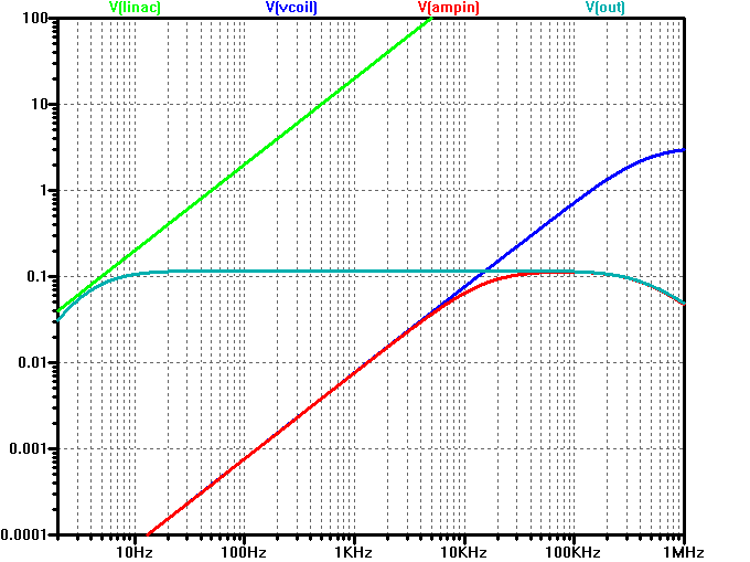
The green curve shows the voltage linac inside the Rogowski model. Note that it reaches 1 V at 50 Hz and increases linearly with frequency.
The blue curve is the green curve scaled so that it has a value of 383 µV at 50 Hz.
The red curve is the input of the amplifier. It follows the blue curve up to just below 10 kHz, where the low-pass action of R3/C3 kicks in and flattens the curve. As mentioned above, this knee is chosen to coincide with the opposite knee of the amplifier caused by R7/C5 so that the total response, the grayish-green curve, is flat from 30 Hz to 100 kHz. The gain is just above 0.1 V/A, which makes this design suitable for applications with up to at least 10 A of maximum current.
One caveat when testing or using this circuit is that it takes a pretty long time for the 100 µF capacitor to charge up via the 2.2 megohm resistor after power up. The time constant here is more than three minutes (220 seconds), which means it will take a long time from power up until the circuit is operational. If this is a problem in any given application, one could consider placing a CMOS switch (like 4066) across the 2.2 megohm resistor and let it be closed for a short period after power up.
The 10 µF capacitor at the input of the amplifier will also take some time to charge. Here the time constant is 5 seconds, so this is less of a problem than the 100 µF cap. This can be improved by reducing the 1 megohm bias resistors to 330k, which will have little effect on the overall response. Even 100k might be acceptable, although this will cause some unevenness in the response above 10 kHz.
In the schematic, the amplifier LTC6088 is present. I chose this as it was a suitable opamp available in the default LTSpice library. There are however many other amplifiers that would do well in this position. Important characteristics are:
- Operation at 5 V
- Preferably rail-to-rail output
- Reasonably low input bias current, preferably below 50 nA or so
- Enough gain-bandwidth for the application, at least a few MHz